The Physics of Light Transport
A Deep Dive into DWDM Architecture, OTN Layers, and Optical Math
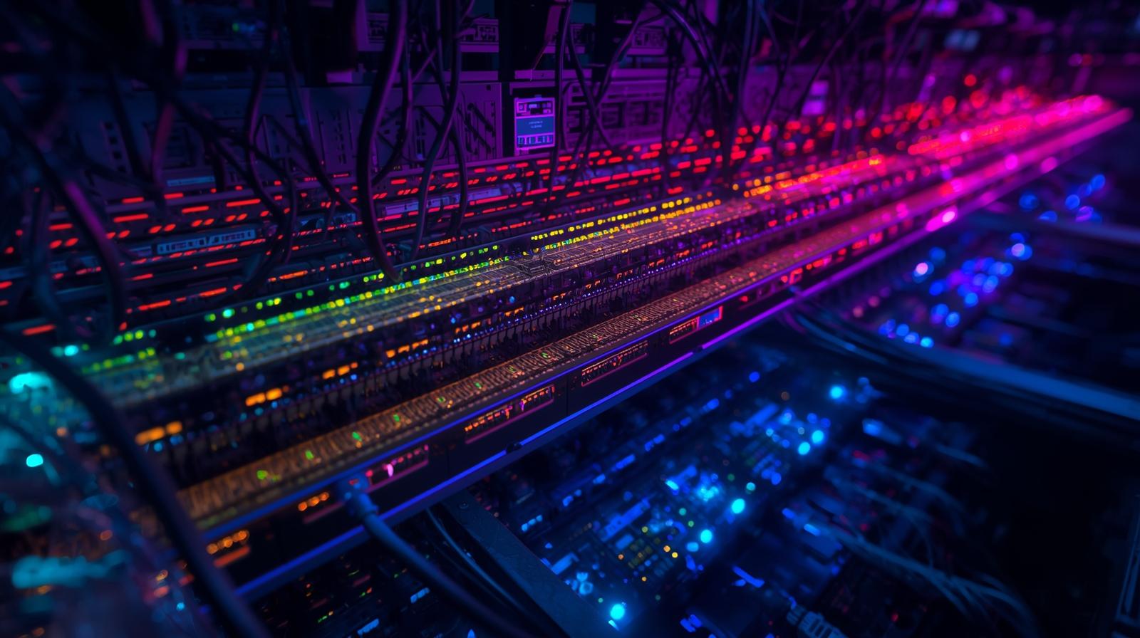
In the world of telecommunications, we often focus on the digital layer—IP packets, MAC addresses, and routing tables. But beneath that digital logic lies the Photonic Layer, a realm governed not by binary code, but by quantum physics, attenuation, and the complex properties of glass.
This guide acts as a comprehensive technical reference for network engineers and architects looking to understand Dense Wavelength Division Multiplexing (DWDM). We will map components to the OSI model, explore the hardware that drives the internet, and break down the mathematical formulas that define the limits of light transport.
1. The Layer Model: OSI vs. Optical (OTN)
While network engineers are trained on the 7-layer OSI model, Optical Transport Networks (OTN) utilize a hierarchy defined by ITU-T G.709. To troubleshoot effectively, you must understand where the “Digital” ends and the “Analog” begins.
Ethernet Frames, IP Packets, Fibre Channel
ODU / OTU / FEC (The “Wrapper”)
Single Wavelength (Lambda)
Combined Wavelengths (ROADM)
Physics: Fiber & Amplifiers
The Breakdown for Troubleshooting
- Client Layer: The payload. At this stage, data is non-deterministic (bursty). Handled by Routers/Switches.
- OTN Layer (L1): The “Digital Wrapper.” Handles Forward Error Correction (FEC). This maps bursty data into a constant-bitrate stream.
- Photonic Layer (L0):
- OCh: If one channel has errors, check the Transponder.
- OMS: If all channels fluctuate, check the ROADM/Mux.
- OTS: If the fiber is cut or dirty, the whole link fails.
2. Component Encyclopedia
Understanding the hardware is essential for network design. Below is a comparison of critical components found in a modern DWDM shelf.
Transponder vs. Muxponder
| Feature | Transponder | Muxponder |
|---|---|---|
| Function | 1:1 Conversion. Maps one client signal (e.g., 100GbE) to one DWDM Wavelength. | N:1 Aggregation. Maps multiple low-speed signals (e.g., 10x 10G) into one high-speed wavelength. |
| Latency | Ultra-low latency (Direct mapping). | Higher latency (Requires buffering/framing). |
| Use Case | High-bandwidth backbone services (400G/800G). | Cost-effective handoffs for lower speed clients. |
CDCF ROADM
The Reconfigurable Optical Add-Drop Multiplexer is the “switch” of the optical world. Modern networks use CDCF architecture:
- Colorless: Any port can accept any wavelength (no fixed filters).
- Directionless: Traffic can be routed to any outgoing fiber direction (North/South/East/West).
- Contentionless: The same frequency can be reused on different directions without blocking.
- Flex-Grid: Supports variable channel widths (37.5GHz to 100GHz+) for modern baud rates.
Amplifiers: EDFA vs. Raman
Light fades as it travels through glass. We use two main types of physics to boost the signal:
- EDFA (Erbium Doped Fiber Amplifier): A “lumped” amplifier. Uses Erbium ions and a pump laser to clone signal photons. High gain (20-30dB), but adds noise.
- Raman Amplifier: A “distributed” amplifier using the transmission fiber itself. A high-power laser is shot backwards into the fiber, transferring energy via Stimulated Raman Scattering. Critical for ultra-long spans.
3. The Mathematics of Transport
You don’t need to be a physicist to design a network, but you must understand the formulas that dictate reach and capacity.
1. The Shannon Limit (Capacity)
This is the theoretical speed limit of data transfer. It dictates why we need higher Signal-to-Noise Ratios (SNR) to achieve higher speeds (like 800G).
- C = Channel Capacity (bits/s)
- B = Bandwidth (Hz)
- SNR = Signal-to-Noise Ratio (linear)
2. Optical Power Budget
Calculated to ensure light reaches the receiver above the sensitivity threshold (usually -30dBm) but below the saturation point.
- Prx / Ptx = Receive and Transmit Power
- Gamp = Total Gain from amplifiers
- Lfiber = Distance (km) × 0.22 dB/km
3. OSNR (Optical Signal to Noise Ratio)
Every amplifier adds noise (ASE). As signals pass through multiple hops, the noise floor rises. If the OSNR drops below the receiver’s threshold, uncorrectable bit errors occur.
Conclusion
Modern optical networks are a marvel of engineering, balancing the raw physics of light with sophisticated digital signal processing. Whether you are configuring a Transponder or calculating a Link Budget, understanding the interaction between the Photonic Layer (L0) and the Digital Layer (OTN L1) is the key to building resilient, high-capacity networks.
Reference: ITU-T G.709, G.694.1, G.975.