
Microwave and Antenna Various Matlab Codes. Some of the Projects are below.
Polar form for a Symmetrical Dipole of Finite Length: Matlab Script
The MATLAB code calculates and plots various quantities associated with a dipole antenna. Here’s a breakdown of its functionality:
- Variable Initialization:
- The code prompts the user to input the length of the dipole antenna in wavelengths.
- It sets the value of
etato 120π, representing the characteristic impedance of free space. - The current amplitude,
I0, is set to 1. - The variable
thetais initialized as an array ranging from 1 to 180 degrees in steps of 1, converted to radians. - The difference between consecutive elements in
thetais stored indth.
- Calculation of Radiation Pattern:
- The code computes the radiation intensity,
U, using the given dipole length (L) andthetavalues. - It determines the maximum radiation intensity,
UMAX. - The radiated power,
Prad, is calculated by summing the product ofU,sin(theta),dth, and 2π. - The code then evaluates the directivity,
D, using the formula(4π*UMAX)/Prad. - The directivity in decibels,
D_db, is computed as10*log10(D).
- The code computes the radiation intensity,
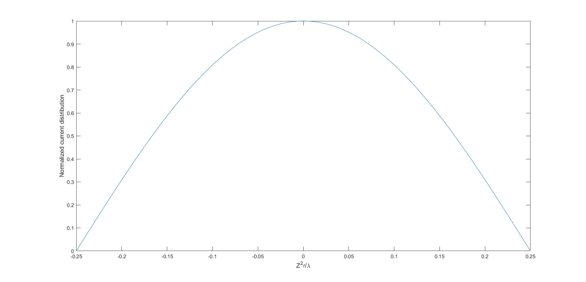
- Calculation and Plotting of Current Distribution:
- The code generates an array,
Z, with 1000 equally spaced points ranging from-L/2toL/2, representing the distance along the dipole. - It calculates the normalized current distribution,
I, based on the givenZvalues. - A plot of the absolute value of
IversusZis created to visualize the current distribution.
- The code generates an array,
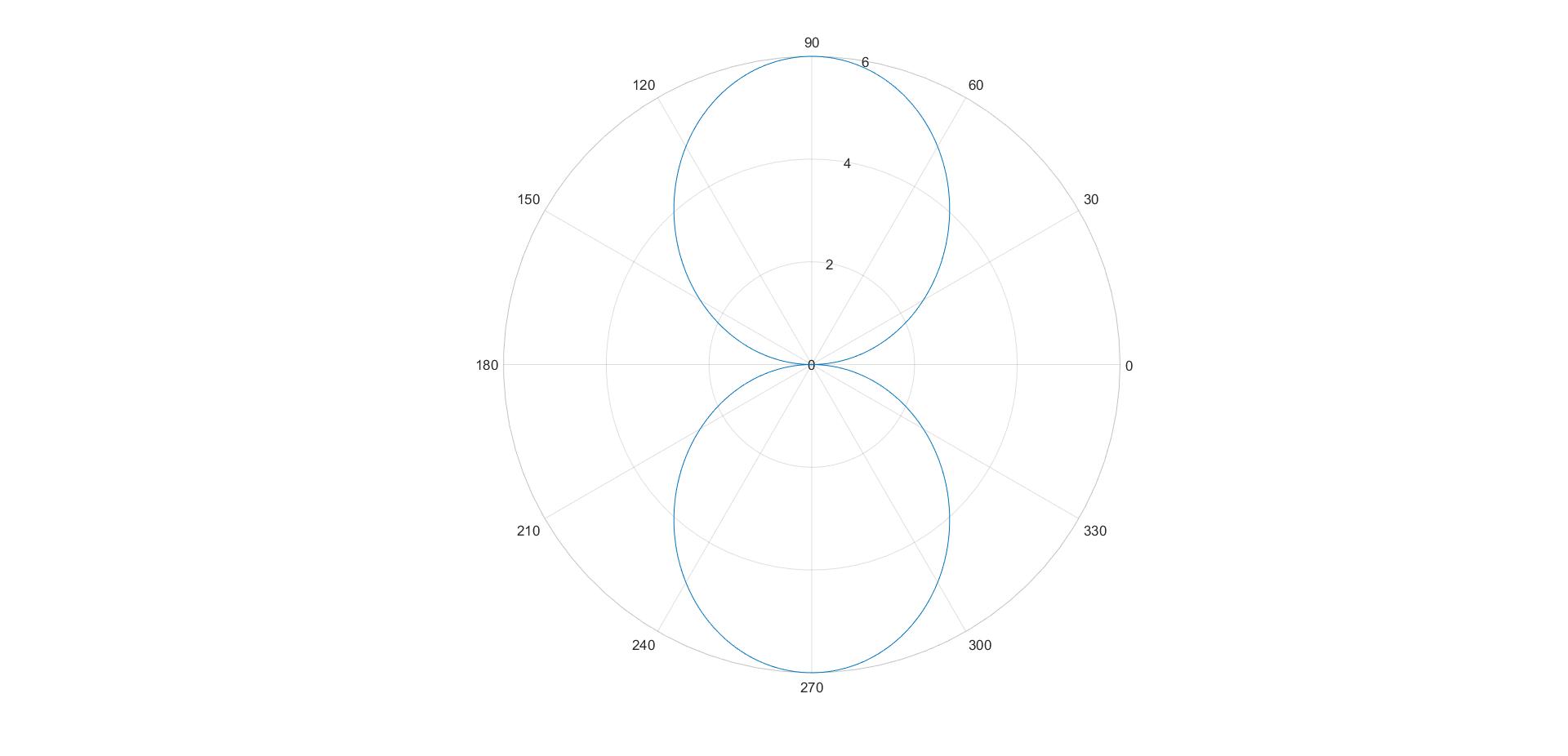
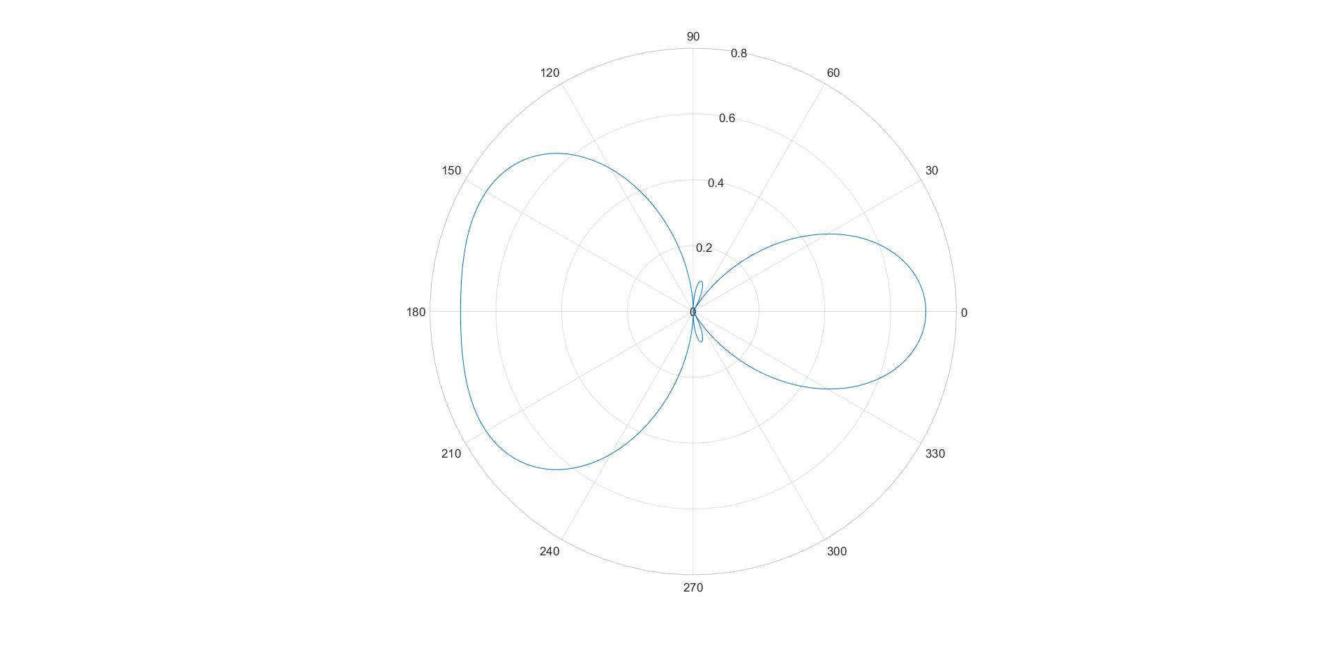
- Calculation and Plotting of Electric Field Pattern:
- The code redefines
thetaas an array ranging from 1 to 360 degrees in steps of 1, converted to radians. - Parameters such as the distance
r(set to 10) and wavelengthlambda(set to 0.3) are initialized. - The wave number,
k, is computed as2π/lambda. - The dipole length,
L, is adjusted tolambda/2. - The electric field strength,
E, is calculated using the dipole antenna formula. - A polar plot of the absolute value of
Eversusthetais created to visualize the electric field pattern.
- The code redefines
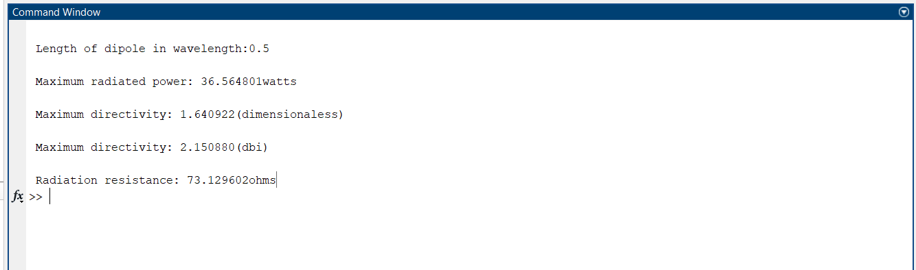
- Printing Results:
- The code displays the maximum radiated power,
Prad, in watts. - It shows the maximum directivity,
D, in dimensionless units. - The maximum directivity,
D_db, is also displayed in decibels. - Finally, the radiation resistance,
Rr, is shown in ohms.
- The code displays the maximum radiated power,
This MATLAB code provides insights into the characteristics of a dipole antenna, including radiated power, directivity, current distribution, and electric field pattern.
clear all; close all; clc;
L = input('\n Length of dipole in wavelength:');

eta = 120*pi;

I0 = 1;
theta = (1:1:180)*pi/180;

dth = theta(2)-theta(1);

U = eta*(abs(I0)^2/(8*pi^2))*((cos((L*pi)*cos(theta))-cos(L*pi))./sin(theta)).^2;

UMAX=max(U);

Prad = sum(U.*sin(theta)*dth*2*pi);

D = (4*pi*UMAX)/Prad;
D_db = 10*log10(D);

Rr = (2*Prad)/(abs(I0)^2);

Z=linspace(-L/2,L/2,1000);
I=sin(2*pi*(L/2-abs(Z)));
figure(1),plot(Z, abs(I));
xlabel('Z^2{\prime}/\lambda','fontsize',12);
ylabel('Normalized current distribution','fontsize',12);

theta = (1:1:360)*(pi/180);
r=10;

lambda=0.3;
k=(2*pi)/lambda;

L=lambda/2;
E=1i*eta*I0*exp(-1i*k*r)*(1/(2*pi*r))*((cos(k*L*cos(theta)/2)-cos(k*L/2))./sin(theta));
figure(2),polarplot(theta, abs(E));

fprintf('\n Maximum radiated power: %fwatts\n',Prad);
fprintf('\n Maximum directivity: %f(dimensionaless)\n',D);
fprintf('\n Maximum directivity: %f(dbi)\n',D_db);
fprintf('\n Radiation resistance: %fohms\n',Rr);
Output
Radiated Power and Maximum Directivity of any Antenna: Matlab code
% Radiated power and Directivity of an antenna:
close all;
clear all;
clc;
format long;
%Angle definition:
%Azimuth angle phi ranges between 0 to 360 degrees:
phi_degree = 0:360;
phi_rad = phi_degree * pi/180; %Converting degrees to radians
%Elevation angle theta ranges between 0 to 180 degres:
theta_degree = 0:180;
theta_rad = theta_degree* pi/180; %Converting degrees to radian
%integration step size:
dth=theta_rad (2) -theta_rad (1);
dph=phi_rad (2) -phi_rad (1) ;
[THETA, PHI] =meshgrid (theta_rad, phi_rad);
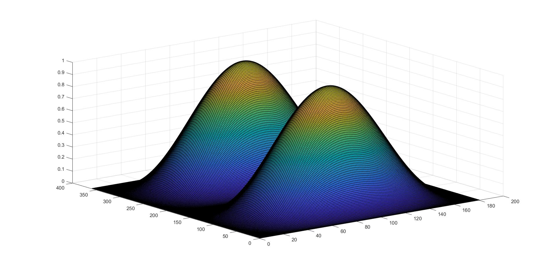
%Radiation pattern of an antenna:
U = (sin (THETA).*sin (PHI) ).^2;
%Performing nunerical integration to obtain
%average power radiated by the antenna:
P_avg=sum(sum (U.*sin(THETA)*dth*dph) );
%Note sum() is discrete time equivalent of integration
%use of sum() twice is to integrate w. r.t. theta and phhi
%Directivity:
%D=4*pi*P_max (theta, phi)/P_avg(theta, phi)
D=4 *pi*max(max (U) )/P_avg;
D_db = 10*log10(D);
fprintf('Average power radiated by the antenna is %f\n', P_avg);
fprintf('Directivity of the antenna is %f(dimensionless) and %f(in dB)\n',D,D_db);
surf(U);Output
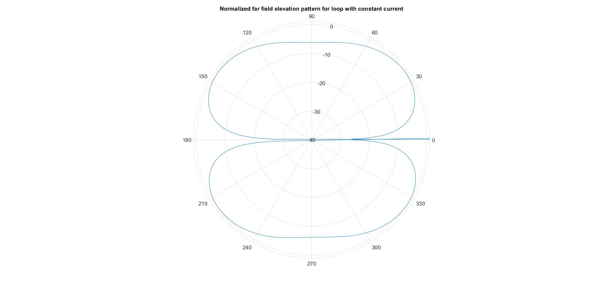
Polar form for a Loop Antenna with Uniform Current: Matlab code
clear all;close all; clc;
format long;
%-Definition of constants and initialization---%
%Free space impedance:
eta = 120*pi;
% Angle vector:
theta=(1:180)*(pi/180);
%Integration step size
dth = theta(2) - theta(1);
%Reading the radius of the loop
A = input ('\nSpecify radius of loop in wavelengths:');
%-------------------------------------------------------
%diation intensity calculation:
%A^2*omega*2 X mu^2 |I0|^2*J1^2(k*A*sin(theta))
%U
%8*eta
%Using omega = 2*pi*f and f = C/lambda,
%C 1/sqrt(mu * epsilon) and eta = sqrt{mu/epsilon) = 120*pi
%Simplified radiation intensity is given by:
% A2*(2*pi*2*eta |I0|^2*J1^2*(k*A*sin(theta))
%----------------------------------------------------------
F = besselj(1,(2.0*pi*A*sin(theta)));
U = A^2*(2*pi)^2*F.^2*eta/8;
%Radiated power:
Prad = sum(2*pi*U.*sin (theta) *dth);
%Directivity:
D = (4.0*pi*max(U))/Prad;
D_dB = 10*log10(D);
%Padiation resistance:
Rr = 2.0*Prad;
%Calculation of eievation pattern:
% -A*k*I0*exp(-jkr)
% H_theta = ----------------------*J1*(k*A*sin(theta))
% 2*r
% Normalized Peak Current
I0 = 1;
%Distance r in neters:
r=10;
% Wavellength in meters:
lambda=1;
%Wave nunber:
k=(2*pi)/lambda;
H_theta=-A*k*I0*exp(-1j*k*r)*besselj(1,k*A*sin(theta))/(2*r);
HdB= 20*log10(abs(H_theta)/max(abs(H_theta)));
HdB = [HdB fliplr(HdB)];
theta = [theta, theta+pi];
figure(1),polarplot(theta,HdB);
title ('Normalized far field elevation pattern for loop with constant current');
rlim([-40 01]);
%Printing the values:
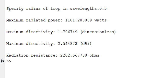
fprintf('\nMaximum radiated power: %f watts\n',Prad);
fprintf(' \nMaximum directivity: %f (dimensionless) \n',D);
fprintf (' \nMaximum directivity: %f (dBi) \n' ,D_dB);
fprintf('\nRadiation resistance: %f ohms\n',Rr);Output
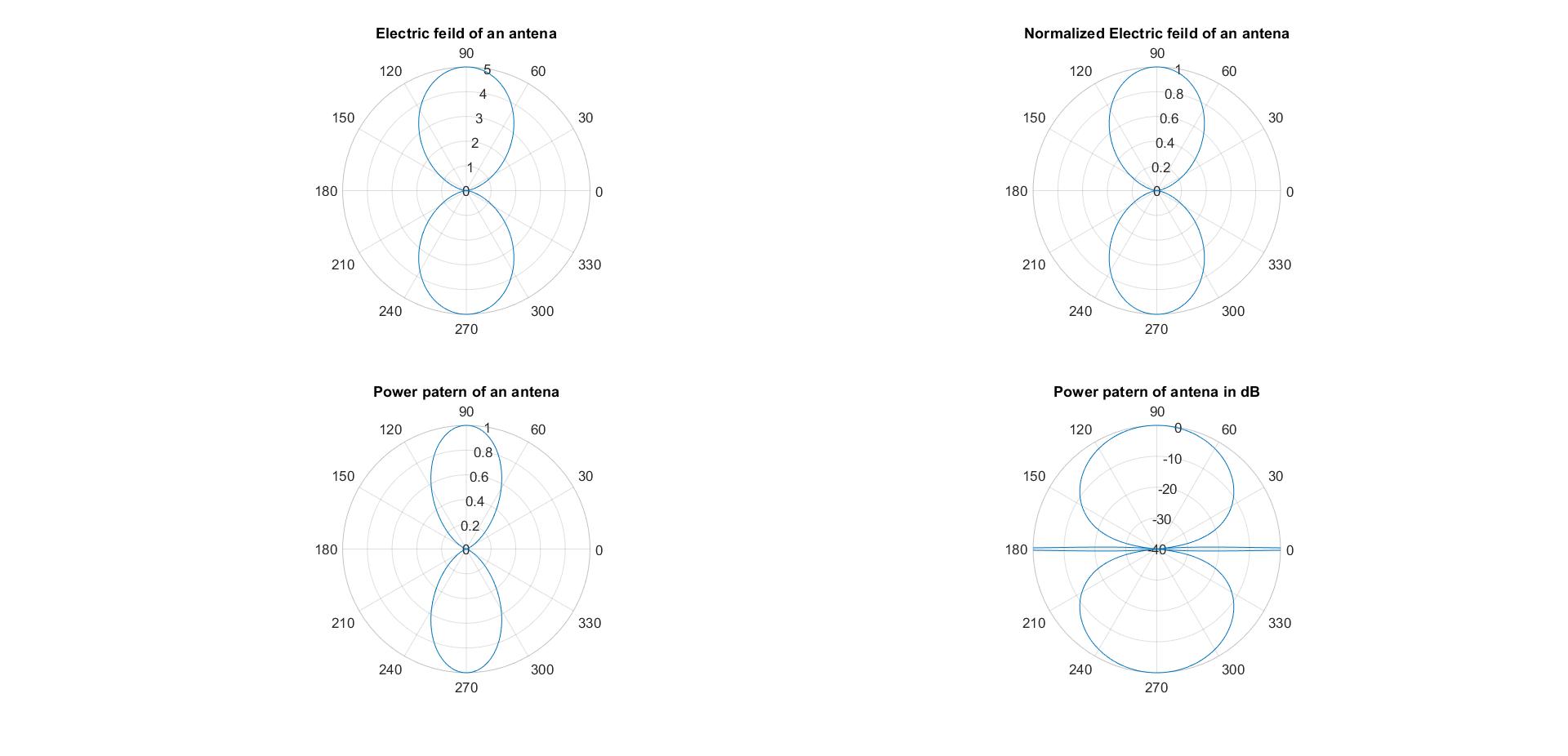
Two Dimensional(2-D) Polar and Semi-Polar Patters using Matlab code
clear all;
close all;
clc;
theta = -pi:0.01:pi; % creation of a angle vector
f = 5*sin(theta).*sin(theta);% electric feild Vector
f_norm = f/max(f);% Normalization (normalized electric feild vector)
power = f_norm.^2;% Power feild
Power_in_db = 10*log10(power);%power in dB
figure(1),
subplot(221)
polarplot(theta,f);
title('Electric feild of an antena');
subplot(222)
polarplot(theta,f_norm);
title('Normalized Electric feild of an antena');
subplot(223)
polarplot(theta,power);
title('Power patern of an antena');
subplot(224)
polarplot(theta,Power_in_db);
rlim([-40,0]);
title('Power patern of antena in dB');
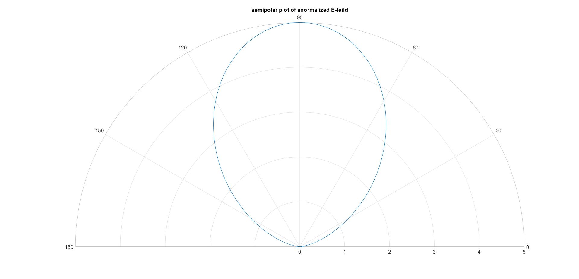
figure(2),polarplot(theta,f);
thetalim([0,180]);
title('semipolar plot of anormalized E-feild');Output
Computing The Radiation Characteristics of Linear Arrays(With MATLAB code), Array factor Equation
clear all;
close all;
clc;
phi = (0:1:360).*(pi/180);
n = input('Enter the number of sources:');
d = input('Enter the spacing between the sources as fraction of wavelength:');
delta = input('Enter the phase differnce between the sources:');
psi = (2*pi*d*cos(phi))+delta;
E = (1/n)*(sin(n*psi/2)./sin(psi/2));
polarplot(phi,abs(E),'Linewidth',3);

%for to get various output plot
%For Plot1: Souces=2, spacing=0.5:0.5, Phase difference=pi/2
%For Plot2: Souces=2, spacing=0.5:0.25, Phase difference=pi/2
%For Plot1: Souces=2, spacing=0.5:0.5, Phase difference=0
%For Plot1: Souces=2, spacing=0.5:0.5, Phase difference=pi
Output
Explore More Projects on Matlab
- Microwave and Antenna Various Matlab Codes
- Multiple Input Multiple Output(MIMO) using Matlab
- Pulse Width Modulation(PWM) working Principal using Matlab
- Quadrature Amplitude Modulation(QAM): Theory and Matlab
- Polar form for a Symmetrical Dipole of Finite Length: Matlab Script
- Radiated Power and Maximum Directivity of any Antenna: Theory and Matlab code
- Polar form for a Loop Antenna with Uniform Current: Theory and Matlab code
- Two Dimensional(2-D) Polar and Semi-Polar Patters using Matlab code
- Computing The Radiation Characteristics of Linear Arrays(With MATLAB code), Array factor Equation
- MATLAB code for Binary Frequency Shift Keying(BFSK) Modulation and Demodulation
Join us for Regular Updates
| Telegram | Join Now |
| Join Now | |
| Join Now | |
| Join Now | |
| Join Now | |
| Join our Telegram | connectkreations |
About Connect Kreations
We the team Connect Kreations have started a Blog page which is eminently beneficial to all the students those who are seeking jobs and are eager to develop themselves in a related area. As the world is quick on uptake, our website also focuses on latest trends in recent technologies and project learning and solutions. We are continuously putting our efforts to provide you with accurate, best quality, and genuine information. Here we also have complete set of details on how to prepare aptitude, interview and more of such placement/ off campus placement preparation.
Connect Kreations is excited to announce the expansion of our services into the realm of content creation! We are now offering a wide range of creative writing services, including poetry, articles, and stories.
Whether you need a heartfelt poem for a special occasion, a thought-provoking article for your blog or website, or an engaging story to captivate your audience, our team of talented writers is here to help. We have a passion for language and a commitment to creating high-quality content that is both original and engaging.
Our services are perfect for individuals, businesses, and organizations looking to add a touch of creativity and personality to their content. We are confident that our unique perspectives and diverse backgrounds will bring a fresh and exciting voice to your project.
Thank you for choosing Connect Kreations for your content creation needs. We look forward to working with you and helping you to bring your vision to life!
The website is open to all and we want all of you to make the best use of this opportunity and get benefit from it..🤓
- Our Websites: Connect Kreations